In this post, we’ll be exploring how well two key offensive stats, Third Down Conversion Rate and Total Yards Gained, can predict whether the Baltimore Ravens won a game. We’ll use Logistic Regression, a standard statistical technique for binary outcomes, to model the probability of a win.
Preprocessing
The data we’ll be using is the 2018-2024 seasons of the Baltimore Ravens which was taken from pro-football-reference.com. I aggregated all 7 seasons into one file which I’ll be using for other statistical analyses.
Since we’re only using a few features, there’s no point in us using the full dataset with dozens of columns when we only need a fraction of them. So what we’re gonna do is extract the columns ‘season’, ‘date’, ‘week’, ‘opp’, ‘total yards’, ‘3rd down made’, ‘3rd down attempted’, and ‘Result’. All of these will be placed into a separate spreadsheet so we can focus on the features relevant for this analysis.
Along with that, we’ll do some feature engineering where we create 2 more columns, WinBinary, and ThirdDownPct, which will also be included in our analysis. WinBinary will serve as a simplified column for the computer to read wins as 1 and losses as 0. Third down percentage can simply be calculated by dividing the third downs made by the third downs attempted.
Every time I try to import only using the file’s name, it doesn’t work. So I prefer to load the file in using the path link which includes the folder(s) the file sits in. You can do this by right-clicking the file in whatever folder it’s in, clicking ‘Copy as path’, then pasting it in the parentheses.
Make sure to include an ‘r’ just before the first quote of the file path. This is needed because Python recognizes backslashes (\) as a particular command and will thus misread the file path. The ‘r’ tells it they are a part of the file.
Preprocessing Code
import pandas as pd# Load your normalized file (adjust path if needed)df = pd.read_csv(r"C:\Users\user\folder\Ravens_2018_2024_Normalized.csv")# --- Create TotalYards df.rename(columns={ 'Tot': 'TotalYards', '3DConv': 'ThirdDownMade', '3DAtt': 'ThirdDownAtt', 'Rslt': 'Result'}, inplace=True)# --- Create WinBinary: 1 for win, 0 for lossdf['WinBinary'] = df['Result'].str.startswith('W').astype(int)# --- Create ThirdDownPct = Made / Att (with zero division handling)df['ThirdDownPct'] = df.apply( lambda row: row['ThirdDownMade'] / row['ThirdDownAtt'] if row['ThirdDownAtt'] != 0 else 0, axis=1)# --- Optional: Reorder columns to match the spreadsheetordered_cols = [ 'Season', 'Date', 'Week', 'Opp', 'Result', 'TotalYards', 'ThirdDownMade', 'ThirdDownAtt', 'WinBinary', 'ThirdDownPct']df = df[ordered_cols]# --- Save outputdf.to_csv("Ravens_2018_2024_WinBinary_3rdDownPct.csv", index=False)print("File saved as 'Ravens_2018_2024_WinBinary_3rdDownPct.csv'")
The Logistic Regression Code
This is the full code of the logistic regression we’re implementing:
import pandas as pdimport numpy as npfrom numpy.linalg import invimport matplotlib.pyplot as pltimport seaborn as snsimport statsmodels.api as smfrom sklearn.metrics import confusion_matrix, ConfusionMatrixDisplayfrom sklearn.calibration import calibration_curve# Load datasetdf = pd.read_csv(r"C:Users\YourUsername\Folder\FileName.csv")# Define features and targetX = df[["ThirdDownPct", "TotalYards"]]X = sm.add_constant(X)y = df["WinBinary"]# Fit logistic regressionmodel = sm.Logit(y, X).fit(disp=0)print(model.summary())df["PredictedProbability"] = model.predict(X)# Binned calibration datadf["PredictedBin"] = pd.cut(df["PredictedProbability"], bins=np.arange(0, 1.1, 0.1), include_lowest=True)calibration = df.groupby("PredictedBin").agg( ActualWinRate=("WinBinary", "mean"), AvgPredicted=("PredictedProbability", "mean")).reset_index()#View results of first 3 gamesdf["LogOdds"] = model.predict(X, which="linear")print(df[["ThirdDownPct", "TotalYards", "LogOdds", "PredictedProbability", "WinBinary"]].head(3))# Track Newton-Raphon iterationsdef run_newton_raphson_until_converged(X, y, tol=1e-6, max_iter=100): beta = np.zeros(X.shape[1]) history = [] for i in range(max_iter): z = X @ beta pi = 1 / (1 + np.exp(-z)) gradient = X.T @ (y - pi) W_diag = pi * (1 - pi) W = np.diag(W_diag) hessian = -X.T @ W @ X update = inv(hessian) @ gradient beta_new = beta - update history.append({ "Iteration": i + 1, "Beta": beta.copy(), "Gradient": gradient.copy(), "Update (Δβ)": update.copy(), "New Beta": beta_new.copy() }) if np.linalg.norm(update) < tol: print(f"✅ Converged at iteration {i + 1}") break beta = beta_new return historyprint("\n--- Newton-Raphson Manual Iterations ---\n")X_np = X.values # Convert to NumPy for matrix mathy_np = y.valuesnr_history = run_newton_raphson_until_converged(X_np, y_np)for step in nr_history: print(f"Iteration {step['Iteration']}") print("Initial β:", step["Beta"]) print("Gradient:", step["Gradient"]) print("Update Δβ:", step["Update (Δβ)"]) print("New β:", step["New Beta"]) print()# 1. SCATTERplt.figure()sns.scatterplot(data=df, x="ThirdDownPct", y="TotalYards", hue="WinBinary", palette="coolwarm")plt.title("Scatter: 3rd Down % vs Total Yards")plt.xlabel("3rd Down Conversion %")plt.ylabel("Total Offensive Yards")plt.show()# 2. HEATMAPdf["TD_bin"] = pd.cut(df["ThirdDownPct"], bins=5)df["Yards_bin"] = pd.cut(df["TotalYards"], bins=5)heatmap_data = df.pivot_table(index="TD_bin", columns="Yards_bin", values="WinBinary", aggfunc="mean")plt.figure()sns.heatmap(heatmap_data, annot=True, cmap="Blues", fmt=".2f")plt.gca().invert_yaxis()plt.title("Heatmap: Win Rate by Binned Efficiency & Yards")plt.xlabel("Total Yards (Binned)")plt.ylabel("3rd Down % (Binned)")plt.show()# 3. CALIBRATION CURVEprob_true, prob_pred = calibration_curve(y, df["PredictedProbability"], n_bins=6)plt.figure()plt.plot(prob_pred, prob_true, marker='o', label="Model")plt.plot([0, 1], [0, 1], linestyle='--', color='gray', label="Perfectly Calibrated")plt.title("Calibration Curve: Predicted vs Actual Win Rate")plt.xlabel("Predicted Win Probability")plt.ylabel("Actual Win Rate")plt.legend()plt.show()# 4. Marginal Effect of 3rd Down Efficiency (Hold TotalYards Constant)# --- Prep ---cov_matrix = model.cov_params() # covariance of β'sz_score = 1.96 # for 95% CIdef sigmoid(z): return 1 / (1 + np.exp(-z))# Range & constanttd_range = np.linspace(df["ThirdDownPct"].min(), df["ThirdDownPct"].max(), 100)mean_ty = df["TotalYards"].mean()# Build exog for marginal effectX_marg_td = pd.DataFrame({ "const": 1, "ThirdDownPct": td_range, "TotalYards": mean_ty})# 1) Log-odds predictionlinear_pred_td = model.predict(X_marg_td, which="linear")# 2) SE on log-odds scalese_td = []for _, row in X_marg_td.iterrows(): se_td.append(np.sqrt(row @ cov_matrix.values @ row.T))se_td = np.array(se_td)# 3) Sigmoid → probability + CIpred_prob_td = sigmoid(linear_pred_td)upper_td = sigmoid(linear_pred_td + z_score * se_td)lower_td = sigmoid(linear_pred_td - z_score * se_td)# 4) Plotplt.figure(figsize=(8,5))plt.plot(td_range, pred_prob_td, color='blue', label='Predicted Win Prob')plt.fill_between(td_range, lower_td, upper_td, color='blue', alpha=0.3, label='95% Confidence')plt.title("Marginal Effect of 3rd Down Efficiency")plt.xlabel("3rd Down Conversion Rate")plt.ylabel("Win Probability")plt.ylim(0,1)plt.legend()plt.grid(True)plt.show()# 5. Marginal Effect of Total Yards (Hold 3rd Down % Constant)# --- Prep (if not already done) ---cov_matrix = model.cov_params()z_score = 1.96def sigmoid(z): return 1 / (1 + np.exp(-z))# Range & constantty_range = np.linspace(df["TotalYards"].min(), df["TotalYards"].max(), 100)mean_td = df["ThirdDownPct"].mean()# Build exog for marginal effectX_marg_ty = pd.DataFrame({ "const": 1, "ThirdDownPct": mean_td, "TotalYards": ty_range})# 1) Log-odds predictionlinear_pred_ty = model.predict(X_marg_ty, which="linear")# 2) SE on log-odds scalese_ty = []for _, row in X_marg_ty.iterrows(): se_ty.append(np.sqrt(row @ cov_matrix.values @ row.T))se_ty = np.array(se_ty)# 3) Sigmoid → probability + CIpred_prob_ty = sigmoid(linear_pred_ty)upper_ty = sigmoid(linear_pred_ty + z_score * se_ty)lower_ty = sigmoid(linear_pred_ty - z_score * se_ty)# 4) Plotplt.figure(figsize=(8,5))plt.plot(ty_range, pred_prob_ty, color='green', label='Predicted Win Prob')plt.fill_between(ty_range, lower_ty, upper_ty, color='green', alpha=0.3, label='95% Confidence')plt.title("Marginal Effect of Total Yards")plt.xlabel("Total Yards")plt.ylabel("Win Probability")plt.ylim(0,1)plt.legend()plt.grid(True)plt.show()# 6. HISTOGRAM OF PREDICTED PROBABILITIESplt.figure()sns.histplot(df["PredictedProbability"], bins=10, color="purple")plt.title("Histogram of Predicted Win Probabilities")plt.xlabel("Predicted Win Probability")plt.ylabel("Count of Games")plt.show()# 7. CONFUSION MATRIXdf["PredictedClass"] = (df["PredictedProbability"] >= 0.5).astype(int)cm = confusion_matrix(y, df["PredictedClass"])disp = ConfusionMatrixDisplay(confusion_matrix=cm, display_labels=["Loss", "Win"])disp.plot(cmap="Blues", values_format="d")plt.title("Confusion Matrix (Threshold = 0.5)")plt.show()
Line-By-Line Analysis
import pandas as pdimport numpy as npfrom numpy.linalg import invimport matplotlib.pyplot as pltimport seaborn as snsimport statsmodels.api as smfrom sklearn.metrics import confusion_matrix, ConfusionMatrixDisplayfrom sklearn.calibration import calibration_curve
As always we’re gonna start with importing the Pandas library, the staple for data manipulation.
Next we import NumPy, which is used for advanced math calculations. Anytime you see ‘np.’ in the code, that’s NumPy being called.
The next NumPy line uses a ‘.linalg’ submodule for linear algebra and also imports ‘inv’ for the matrix inverse function. This will be used in the Newton-Raphson iterations.
Next we import matplotlib which is the standard library for visualizations. In the last section of the code we’ll see lots of ‘plt.’ which is the command for the visualizations/graphs we’ll be doing.
Seaborn is simplified subset of matplotlib that’s specialized for custom graphs. ‘sns’ is its shorthand command.
Statsmodels API is the main library that’ll be used for the logistic regression.
And lastly we’re importing two special visualizations from the sci-kit learn library, confusion matrix and calibration curve.
df = pd.read_csv(r"C:Users\YourUsername\Folder\FileName.csv")
We load in our 7-season spreadsheet file. We’re using a csv format instead of xlsx since csv’s load much faster, even though they take up more space. ‘df’ stands for DataFrame which is pandas’ own form of spreadsheet that it will hold our dataset in. ‘df’ is just a common sense variable name we’re using, but it can be what ever you want it to be. Any time you see ‘df’ in this script, that means we’re calling our dataset.
X = df[["ThirdDownPct", "TotalYards"]]X = sm.add_constant(X)y = df["WinBinary"]
We use the ‘X’ variable to declare our selected quantitative predictors, ‘ThirdDownPct’ and ‘TotalYards’. ‘df’ calls for our dataset that has these features, and of course the brackets contains them into a subset to ensure those are the only features that are focused on. These are our independent variables.
In the next line, we use the ‘sm’ alias which calls the statsmodels.api library that we imported. We follow that with ‘add_constant'(X). This assigns a column of 1s into the subset we just made so the model can learn an intercept term, which is a baseline prediction if all other variables are at 0. If we did not do this, the model would assume the probability of winning is 0.5 even if both of those features are 0, which is unrealistic. You are absolutely not winning a game with 0 total yards and you’re super unlikely to win with 0 third down conversions.
Then we declare our response vector, which is ‘WinBinary’. The model will recognize wins as 1 and losses as 0. This is vital for logistic regression since we’re working with binary either-or outcomes
model = sm.Logit(y, X).fit()
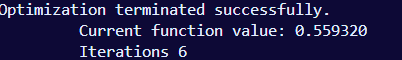
This is the actual initialization of logistic regression. Everything after this will be tuning the model. We’ll use common sense and call this variable ‘model’. Again, we use ‘sm’ to call for the statsmodels.api module, and we access the Logit class inside of it which is literally logistic regression. We set the argument y and X for our binary response vector and our design matrix with our predictors that we just went over. The model is currently unfitted, so we then follow with the ‘.fit’ method which applies maximum likelihood estimation (MLE) to find the optimal β coefficients (intercept and slopes) that maximize the probability of observing the given outcomes. Again, MLE maximizes the likelihood function, but in this case, we’re use negative log-likelihood since this model is using the Newton-Raphson optimization algorithm which minimizes the functions. The method also displays the current function value which is the negative log-likelihood at the final iteration which is called convergence. Convergence is simply when the optimization algorithm has reached a point where updates to the β coefficient are so small there’s no noticeable difference in the negative log-likelihood.
print(model.summary())
This will output the results of the model’s implementation
df["PredictedProbability"] = model.predict(X)
In the same way we selected our two features a few lines back, this line does the same, except it’s creating a new feature since ‘PredictedProbability’ is not already in it. On the right side of this line, we call our ‘model’ variable and use a ‘.predict’ method with it which will return the predicted probabilities, which is the primary result we’re looking for. We want to see the probability of a win given our selected features. This line is set up to establish that output for us when the analysis is done. And lastly, we use ‘X’ as an argument since that is the variable that contains our two selected features, ThirdDownPct and TotalYards.
df["PredictedBin"] = pd.cut(df["PredictedProbability"], bins=np.arange(0, 1.1, 0.1), include_lowest=True)
We’re creating a new column called ‘PredictedBin’ that will hold the results of the predicted probabilities as they’re categorized into various intervals.
We assign that to a pandas’ method called ‘.cut’ which converts continuous numerical data into discrete categories. Its argument will be ‘PredictedProbability’. Since probability is by default continuous (ranging from 0-1), we are binning it into intervals (0.1, 0.2, etc). The second argument uses a NumPy array of those intervals, which are the bin’s edges. 0 is where the bin will start, 1.1 is where it will go up to but not include, so it’ll actually stop at 1.0, and 0.1 is the increment it will go up each time (0.1, 0.2, 0.3,…)
Though not specified in the code, the ‘arange’ method by default is a half-open arrange, meaning the argument does not include the edges as we just went over. This helps avoid overlapping intervals in the case where if we had bins 0.0-0.1 and 0.1-0.2, then where would 0.1 go?
Lastly, the ‘include_lowest’ line simply ensures that 0.0, the lowest value is included in the first bin. Otherwise it’d be starting at 0.1.
calibration = df.groupby("PredictedBin").agg( ActualWinRate=("WinBinary", "mean"), AvgPredicted=("PredictedProbability", "mean")).reset_index()
We’ll name this variable ‘calibration’ which will observe how well the predicted probabilities are aligned with the actual outcomes. The ‘groupby’ method will point this function to our full DataFrame along with the ‘PredictedBin’ column we just created, and it groups each row by bin label (0-10%, 10-20%, …, 90-100%).
Each bin will have two calculated values. The first will be ‘ActualWinRate’ which will contain the ‘WinBinary’ and the mean proportion of those wins. Meaning if 7 out of 10 games were wins, that’s a 70% win rate for that particular bin. Then there’s ‘AvgPredicted’ which tells you what the model thought the average win probability was for that group. The features ‘PredictedProbability’ and, again, the mean will be used in this bin.
Lastly the ‘.reset_index()’ will convert the grouped result back into a flat DataFrame with ‘PredictedBin’ as a regular column. Remember we had to create that column, so making it a regular column and not an addition will make for better plotting.
#View results of first 3 gamesdf["LogOdds"] = model.predict(X, which="linear")print(df[["ThirdDownPct", "TotalYards", "LogOdds", "PredictedProbability", "WinBinary"]].head(3))
Lastly we’re going to print the results of the first 3 games which we’ll be using in our math breakdown later.
Tracking the Newton-Raphson Iterations
This next section of the code will track the Newton-Raphson iterations that will illustrate the ‘learning’ part of machine learning. What we’ll be seeing is how the coefficients update with each iteration until they’re as accurate as possible.
I recommend skipping ahead to the mathematical breakdown of the Newton-Raphson algorithm so you can see what’s going on under the hood. I will NOT be doing a line-by-line analysis of this section as it isn’t necessary for the model to run. I only included it to illustrate how the algorithm works through the iterations.
Math Breakdown
Step 1: Define the Model
Our goal is to measure the probability of the Ravens getting a win based on their 3rd down conversion rate and total yards in a game. The outcome of a game is binary, either a win or a loss. Since it’s binary, we are classifying wins as 1 and losses as 0.
We have our two predictor variables:
- x1: 3rd down conversion percentage
- x2: total offensive yards gained
And our response variable yi:
- y: the outcome, a win or loss
- i: the given game that’s being evaluated
Logistic regression models the probability of a win as: p(y=1 | x1, x2) = ?
What is the probability the Ravens will a game given the conditions of 3rd down conversion rate and total yards gained?
This probability is determined by three coefficients:
- β0: Intercept (baseline log-odds when the predictors’ values are 0).
- β1: effect of 3rd down conversion percentage on log-odds
- β2: effect of total yards on log-odds
Together, these form the linear combination: z = β0 + β1x1 + β2x2
The z value represents the log-odds of winning. Log-odds are the raw scores that the logistic regression model is calculating; it’s the dough before the bread. On the surface, the numbers displayed by log-odds have little meaning, but just know that they’re necessary for determining the probability as precisely as possible. We will later transform the log-odds into a readable probability (good ole percentages) using the sigmoid function.
Step 2: Linear Combination
Once we’ve defined our model and variables, the first actual calculation logistic regression makes is the linear combination of predictors:
z = β0 + β1x1 + β2x2
We just went over z, which is the raw log-odds; the uninterpretable version of the probability.
- β0: Intercept (baseline log-odds when the predictors’ values are 0).
- β1: effect of 3rd down conversion percentage on log-odds
- β2: effect of total yards on log-odds
The x-variables remain their assigned values, and the β-variables are the coefficients of the x-variables. A coefficient (also called ‘weights’) is the variable’s ‘effect’ on log-odds of winning.
We’re essentially weighing each variable by how much it impacts the outcome of a game, particularly on a logarithmic odds scale.
The coefficients are calculated from the MLE application to the dataset, which includes all games. It tries to match the predicted probabilities to the actual wins and losses, testing its effectiveness. Of course it’s not perfect, but it gets as close as possible, hence probability.
One thing that took me a long time to finally realize, is that these coefficients are not calculated in a conventional algebraic form. It’s not like we have a cookie-cutter equation where we plug the values into the variables and simply solve, it doesn’t work that way in this case. These coefficients are results from an iterative algorithm called Newton-Raphson.
Once we have the coefficient results, we plug them into the linear combination equation, then put that through the sigmoid function and the result of that gives us both the predicted probability with the actual outcome of each game.
Step 3: Logistic Function
Now that we have our log-odds scores (z) for each game, we need to transform them into something more useful: probabilities between 0 and 1.
This is where the sigmoid function comes in. The sigmoid takes any real number and “squashes” it into a range between 0 and 1. It’s defined as:
σ(z) = 1/1+e–z “Sigma of z, or ‘σ(z)’, means take the number z, make its negative, then raise Euler’s number e to that power. Add 1 to this result, then divide 1 by the total. The output is a number between 0 and 1, which represents the predicted probability of a Ravens win.”
A log-odds of 0 is a 50% chance of winning. A positive log-odds (z > 0) is greater than 50%, and a negative (z < 0) is less than. Going off of that principle alone can give us an idea of the chance, but we want to get more precise. Otherwise that’s no different from saying the Ravens are more or less likely to win.
Let’s apply the log-odds from the first 3 games to the sigmoid function and see if the resulting predicted probability matches the one in the output
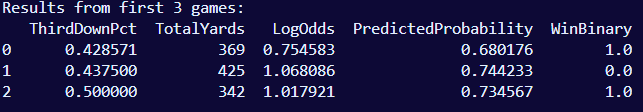
Euler’s number is 2.718281 and infinitely continues, but we’ll stick with 6 decimal places. We set that to the power of our log-odds 0.754583, whose result is 0.470206, which we’ll round to 0.4702. That was the hard part. Now we plug that into the sigmoid function:
1/1+0.4702 = 1/1.4702 = 0.680179, which is just about the same as the computer’s calculation of 0.680176. That only happened since different calculators have their own rounding errors. Regardless, both numbers round to 68%
So now that we’ve used the sigmoid function to get our predicted probabilities, how do we know if our model’s predictions are any good?
Step 4: Likelihood Function
The linear combo gave us the log odds, we put the log odds into the sigmoid, then take the result of the sigmoid, which is the predicted probability, and put that through the likelihood function.
With the likelihood function, we’re measuring how likely the model (with its predictions) were matched to the actual game outcomes
All we’re doing is taking the predicted probability of each game. If the game was a win, the probability stays. If the game was a loss, we subtract that probability from 1. For example, Game 2’s probability was 0.7442. So since that game was a loss, we subtract that 1 – 0.7442 which results in 0.2558.
We calculate the likelihood of observing all the real outcomes using the predicted probabilities. The ‘L’ is the likelihood function which multiplies the chance of every outcome. The ‘∏’ is the product notation which multiplies terms for all the games i=1 to n.
We take the likelihood terms of every game, multiply them, and the product will be our final likelihood function. Which leads us to our next issue:
Step 5: Log-Likelihood
Once we multiply all of those likelihood terms, which are small decimals, our resulting number will be a very small decimal only a few steps away from 0. Something like 0.00000841, which isn’t interpretable.
This is where log-likelihood comes in. This converts the likelihood function into a ‘real’ number that we can do something with.
We’re not gonna get into the deep math of log since it gets messy. We just need to understand its function. Log is basically the opposite of an exponent.
It must be noted that we’re using natural log, not base-10 log. Most calculators’ ‘log’ symbol uses base-10. Make sure you’re using natural log, symbol shown as ‘ln’, before you make that calculation.
So yup. We just take the log-likelihood of each game, add them all together, then our sum is our total log-likelihood
Now that we have the total log-likelihood, which is -64.881, what do we do with it? We test its significance against our log-likelihood of the null model, which is -73.365. We do this by calculating the pseudo-R2 formula which will be the quotient of the LL/LL-null subtracted from 1. The quotient is 0.8844, which subtracted from 1 equals 0.1156.
The ultimate answer is that our model improves log-likelihood by 11.56% compared to the null model. This means our application of two variables to predict a win is somewhat impactful, but of course not a lot. As a rule of thumb in McFadden’s R2, 0.2 – 0.4 is the ideal range for a well fitting model. Below 0.1 is a weak fit which isn’t much different from guessing, and over 0.4 is ‘too’ confident which usually means an error was made in the analysis. So our 0.1156 is, admittedly, a little underwhelming.
Gradient (1st derivative)
For each of the 3 coefficients, we first compute the residual, which is the win binary (1 or 0) minus the predicted win probability, then multiply the residual by the respective feature’s value
Let’s say Game 1 had a 3rd down % of 0.45, total yards of 340, it was a win (which denotes a 1), and the predicted probability was 0.7003. The residual is the win binary minus the predicted probability (yi – πi), 1 – 0.7003 which equals our residual of 0.2997. If the game’s outcome was a loss, it’d be 0 – 0.7003. This is what we are doing for all games.
Once we have all the games’ residuals, we then take them and, in separate equations, multiply them by each feature. So first for the intercept, we multiply every residual by a simple 1; which is 1(0.2997) for Game 1. For the 3rd down pct, we multiply each residual by the respective game’s value for that, which was 0.45 for Game 1. So that’d by 0.45(0.2997) for just Game 1. And we do the same for the total yards, which was 340 for Game 1, making 340(0.2997).
With each feature as its own equation, we do these calculations for all games, and simply add them all together. The resulting answer, our gradient vector, will be a matrix with the 3 sums stacked on top each other.
Hessian (2nd derivative)
The Hessian tells us how fast the gradient is changing with respect to the coefficients. In other words, while the gradient points us in the right direction, the Hessian tells us how steep or flat the surface is, so we can adjust our step size.
In doing this, we build a weight matrix (W)
Each element of W is a game’s predicted probability multiplied by its complement. The complement simply being the predicted prob subtracted from 1. So since Game 1’s predicted prob was 0.7003, its complement is 0.2997, which, when multiplied, equals 0.2099, the ‘weight’ of Game 1.
We put Game 1’s weight against a matrix of the features which are multiplied within each other

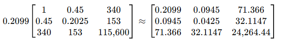
This is the matrix for Game 1. We do this for all games, add all of their matrices, and the result will be a final matrix of the same size, but it’ll contain the sums of all the games.
All of this happens under the table, so we won’t be seeing that final matrix.
Newton-Raphson Algorithm
The whole math process we just did is recalculated with each iteration
We are iterating (or updating) the coefficients (β) to be more accurate. A loop of sorts
The first iteration treats all 3 coefficients as [0,0,0] as a baseline. This means the model has no prior knowledge of previous game data, which means the probability can’t be anything more than a wild guess, which is 50%; they may win, they may not. This makes the model blatantly wrong.
In the first iteration, we take the gradient and compare the predicted probability (which is 0.5 for everything right now) with the actual outcomes for each game. The residuals are large since the model is ignorant. Then we calculate the Hessian which measures how confident the model was in its predictions. Once those two derivatives are computed, the algorithm updates the coefficients to be more accurate. These iterations happen repeatedly until the updates don’t change any more, meaning it’s gotten as accurate as possible, which is convergence. All of this is happening under the hood, there’s nothing in the outputted results that shows how much the updates have changed. We only know it did its job because of ‘converged’ showing ‘True’. Yet I included a section where we track the iterations so we can see them update in real time.
Tracking the Iterations
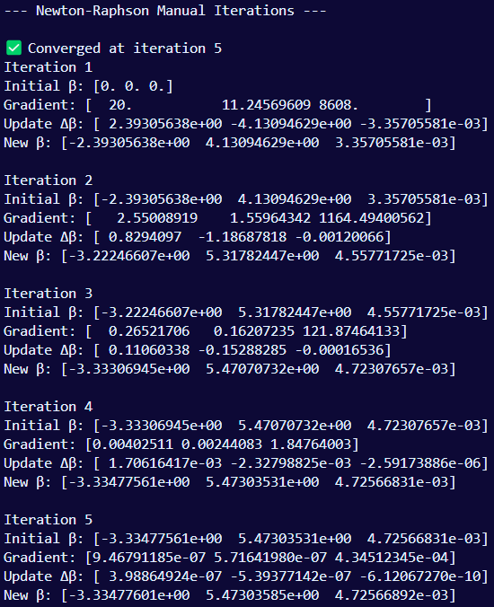
Again, in the first iteration, the model starts all the coefficients blindly at 0.
The updated coefficients after the first iteration is [-2.39, 4.13, 3.36]. After the second iteration, it goes to [-3.22, 5.32, 4.56]. There were a total of 5 iterations, so in the last one, which we have in our final output [-3.33, 5.47, 4.73].
We’re not going to get too deep into the math for this part.
β₀, the intercept, decreased from -2.39 in the first iteration to -3.33 in the final iteration. This shift downward helped balance the upward movement of the other two coefficients. Since the intercept reflects the baseline log-odds of winning when both predictors are 0, this drop means the model adjusted its baseline downward to compensate for the increasing influence of the actual predictors. It ensures that the predicted probabilities still stay within a realistic range (between 0 and 1) as the model becomes more confident in the features.
B1, 3rd down % increased significantly, jumping from 4.13 in the first iteration to 5.47 in the final iteration, which shows that it’s a strong predictor of winning.
B2, total yards, had a lesser, but still decent increase from 3.35 to 4.72, showing that it’s a moderate predictor of winning
Results Breakdown
This is what outputs in the terminal after running the script.
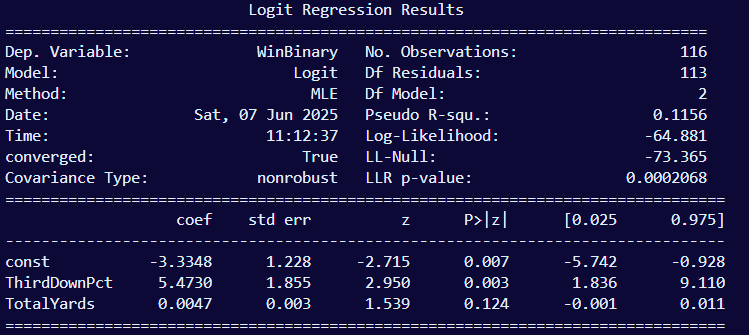
Model Information
- Dependent Variable: ‘WinBinary’; we’re predicting if 2 variables, 3rd down conversions and total yards in this case, predicts wins or losses, which is a pair of binary outcomes. 1 means win and 0 means loss
- Model: ‘Logit’ which is shorthand for logistic regression
- Method: ‘Maximum Likelihood Estimation (MLE)’
- Date & Time: When this analysis was executed
- Converged: The algorithm successfully found a set of coefficient values (βs) that maximize the log-likelihood function; this means the model is stable, hence why it says ‘True’. If it was ‘False’, that means the model is unstable which could be due to a number of factors
- Covariance type: this measures how well the standard errors were calculated. ‘nonrobust’ is the default value, meaning the model is correctly specified and errors meet all assumptions.
- No. Observations: The amount of observations in our data set; the games we’re taking data from, which is 116 since we’re doing the last 7 seasons
- Degrees of freedom (Df Residuals): This value is the number of observations (116 games), minus the number of predictors (2, as showin in Df Model), minus an extra 1 to account for the intercept. This is not to say we’re ‘deleting’ 3 games, it’s that the predictors take away from the flexibility of the dataset. A rule of thumb for the Df Residual is you generally want it to be at least 50, ideally greater than 100. Less than 50 is dangerously unstable, and 100+ is very stable, thus more accurate.
- Df Model: number of predictors used in the model. We’re only using 3rd down % and total yards, which is only 2 predictors
Fit Quality
- Pseudo R-square: logistic regression does not use squared errors (R2) like linear regression does, so we use a pseudo R2 to illustrate how well the model performs relative to a null model. We used McFadden’s R2 in this case. Its interpretive value should generally hover around 0.20, ideally higher than 0.30. Less than 0.20 indicates weak explanatory power, and above 0.30 means a strong fit. Though a strong fit is not typical for logistic regression since it deals with binary outcomes. Our model’s Pseudo R2 is 0.1156, which is actually typical since we’re dealing with binary outcomes and especially since we’re only using 2 predictors
- Log-Likelihood: It works by assigning probabilities to each game outcome based on the current model’s predictions. If a game was a win and the model predicted a high probability of a win, it’s rewarded. If it predicted the opposite, it’s penalized. This score is based on multiplying the probabilities across all games (then taking the log so it doesn’t underflow). The higher (less negative) this value, the better your model fits. In our case, the log-likelihood is –64.881, which is the value our model achieved after the optimizer (Newton-Raphson) climbed the likelihood hill and settled at the best βs.
- LL-Null: This is the log-likelihood of a “dumb” model, one that only uses an intercept and ignores all predictors. It’s like saying: “Let’s just always guess the average win rate, no matter the 3rd down % or yards.” This is the baseline score. Ours is –73.365, which is worse than our model’s log-likelihood (–48.016). That’s what we want, it means our predictors actually improved things.
- LLR p-value: This is the Likelihood Ratio Test. It takes the difference between our full model and the null model and asks: “Is this improvement statistically significant, or could it just be random chance?”. Then it compares that to a chi-square distribution with degrees of freedom equal to the number of predictors. In our case, the LLR p-value is 0.0002068, which means there’s strong evidence that our model is better than guessing the average win rate. This tells us that our predictors matter.
- Coef: These are the final βs we found through MLE. Each one tells us how much its variable influences the log-odds of winning, not the raw probability.
- The intercept (–3.3348) is the baseline log-odds when all other variables are 0.
- 3rd Down % (5.4730) is strongly positive — higher conversion rates dramatically increase win odds.
- Total Yards (0.0047) is a much smaller effect — adds a bit to the log-odds, but not much.
- Std err: This is how uncertain we are about each β. It’s based on the curvature of the log-likelihood peak (aka the Hessian). A smaller standard error means we’re more confident in that β.
- Z: This is the test statistic: each β divided by its standard error (Z = coef/std err). It tells us how many standard deviations away from zero each β is. The bigger the z, the stronger the evidence that the predictor has an effect.
- P>|z|: This is the p-value for each β. It tells us: “If this predictor had no real effect (β = 0), what’s the chance we’d get a z-score this extreme just by luck?” A p-value less than 0.05 usually means we consider it statistically significant.
- [0.025 & 0.975]: This is the 95% confidence interval for each coefficient. It gives us a range where we believe the true β is likely to fall.
Visualizations
Now that we have completed the analysis, we want to see what the results actually mean. As of now all we have is that ugly terminal output that shows a bunch of terms and numbers.
For logistic regression, we’re going to be using 7 types of graphs to illustrate our results.
Scatter Plot
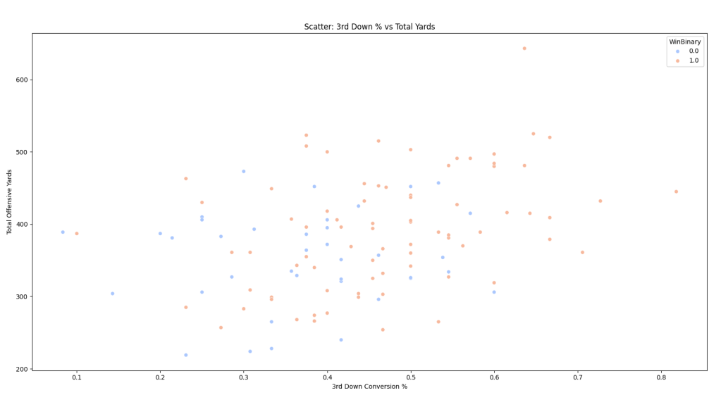
plt.figure()sns.scatterplot(data=df, x="ThirdDownPct", y="TotalYards", hue="WinBinary", palette="coolwarm")plt.title("Scatter: 3rd Down % vs Total Yards")plt.xlabel("3rd Down Conversion %")plt.ylabel("Total Offensive Yards")plt.show()
We’ll kick this off with a scatter plot, one of the more common graphs. This is more exploratory, gives us an overview of the data without having to stare at numbers.
This visual shows the relationship between our two predictors and how much they overlap. Orange dots are wins and blue dots are losses. The x-axis is 3rd down conv. and the y-axis is total yards.
We see the data points are scattered pretty widely. Generally we should be seeing the wins tend towards the upper-right corner and losses towards the bottom-left.
Common sense can tell us that a game with a low amount of total yards is more likely to be a loss. The league average total yards per game is usually a little above 300. The graph reflects that showing only handful of games won below 300.
Heatmap
# 2. HEATMAPdf["TD_bin"] = pd.cut(df["ThirdDownPct"], bins=5)df["Yards_bin"] = pd.cut(df["TotalYards"], bins=5)heatmap_data = df.pivot_table(index="TD_bin", columns="Yards_bin", values="WinBinary", aggfunc="mean")plt.figure()sns.heatmap(heatmap_data, annot=True, cmap="Blues", fmt=".2f")plt.title("Heatmap: Win Rate by Binned Efficiency & Yards")plt.xlabel("Total Yards (Binned)")plt.ylabel("3rd Down % (Binned)")plt.show()
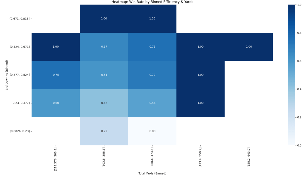
In this graph, total yards is our x-axis, and 3rd down conv. is our y-axis. Each grid in the heatmap shows the probability of a win relative to our two variables. The amount of blue is to proportional to said probability. Both axes are using bins, which are ranges of the values.
Again, using common sense, there’s a low chance of winning if the Ravens have low total yards and a low 3rd down conv. If we look at the variables pulling all of the weight, we see our first tastes of a 1.0 win probability at the 52% 3rd down conv and the 473 total yard bins. One big thing I need to emphasize is that a 1.0 win probability is not the same as a 100% guaranteed win. It simply means that all games with both of those metrics were wins. So in a way, it does give some predictive power, but it’s still not wise to use 1.0 as a 100% chance of winning.
Calibration Curve
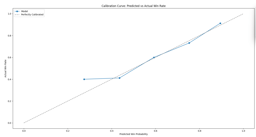
prob_true, prob_pred = calibration_curve(y, df["PredictedProbability"], n_bins=6)plt.figure()plt.plot(prob_pred, prob_true, marker='o', label="Model")plt.plot([0, 1], [0, 1], linestyle='--', color='gray', label="Perfectly Calibrated")plt.title("Calibration Curve: Predicted vs Actual Win Rate")plt.xlabel("Predicted Win Probability")plt.ylabel("Actual Win Rate")plt.legend()plt.show()
A calibration curve simply illustrates how correct our model was in predicting a win versus actual wins.
The straight dotted line is the ideal curve which means the model was 100% in predicting all wins. The blue line with hard points is the model’s predictions. We see the first point is at a 0.3 predicted win probability but the actual win rate was a 0.4. So this means the model started off pessimistic. In the middle to upper ranges it’s pretty accurate, yet it get a bit overconfident at the very top.
Marginal Effects
cov_matrix = model.cov_params() # covariance of β'sz_score = 1.96 # for 95% CIdef sigmoid(z): return 1 / (1 + np.exp(-z))# Range & constanttd_range = np.linspace(df["ThirdDownPct"].min(), df["ThirdDownPct"].max(), 100)mean_ty = df["TotalYards"].mean()# Build exog for marginal effectX_marg_td = pd.DataFrame({ "const": 1, "ThirdDownPct": td_range, "TotalYards": mean_ty})# 1) Log-odds predictionlinear_pred_td = model.predict(X_marg_td, which="linear")# 2) SE on log-odds scalese_td = []for _, row in X_marg_td.iterrows(): se_td.append(np.sqrt(row @ cov_matrix.values @ row.T))se_td = np.array(se_td)# 3) Sigmoid → probability + CIpred_prob_td = sigmoid(linear_pred_td)upper_td = sigmoid(linear_pred_td + z_score * se_td)lower_td = sigmoid(linear_pred_td - z_score * se_td)# 4) Plotplt.figure(figsize=(8,5))plt.plot(td_range, pred_prob_td, color='blue', label='Predicted Win Prob')plt.fill_between(td_range, lower_td, upper_td, color='blue', alpha=0.3, label='95% Confidence')plt.title("Marginal Effect of 3rd Down Efficiency")plt.xlabel("3rd Down Conversion Rate")plt.ylabel("Win Probability")plt.ylim(0,1)plt.legend()plt.grid(True)plt.show()# 5. Marginal Effect of Total Yards (Hold 3rd Down % Constant)# --- Prep (if not already done) ---cov_matrix = model.cov_params()z_score = 1.96def sigmoid(z): return 1 / (1 + np.exp(-z))# Range & constantty_range = np.linspace(df["TotalYards"].min(), df["TotalYards"].max(), 100)mean_td = df["ThirdDownPct"].mean()# Build exog for marginal effectX_marg_ty = pd.DataFrame({ "const": 1, "ThirdDownPct": mean_td, "TotalYards": ty_range})# 1) Log-odds predictionlinear_pred_ty = model.predict(X_marg_ty, which="linear")# 2) SE on log-odds scalese_ty = []for _, row in X_marg_ty.iterrows(): se_ty.append(np.sqrt(row @ cov_matrix.values @ row.T))se_ty = np.array(se_ty)# 3) Sigmoid → probability + CIpred_prob_ty = sigmoid(linear_pred_ty)upper_ty = sigmoid(linear_pred_ty + z_score * se_ty)lower_ty = sigmoid(linear_pred_ty - z_score * se_ty)# 4) Plotplt.figure(figsize=(8,5))plt.plot(ty_range, pred_prob_ty, color='green', label='Predicted Win Prob')plt.fill_between(ty_range, lower_ty, upper_ty, color='green', alpha=0.3, label='95% Confidence')plt.title("Marginal Effect of Total Yards")plt.xlabel("Total Yards")plt.ylabel("Win Probability")plt.ylim(0,1)plt.legend()plt.grid(True)plt.show()
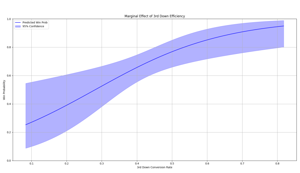

While every other graph observes both variables, marginal effect graphs allow us to see how much a single variable contributes to the predictive probability. This is done by holding the other variable at its constant average. So if we want to observe 3rd down efficiency’s impact, we’ll hold Total Yards at its average, then we do the same for observing Total Yards, holding 3rd down efficiency at its average.
The line is the predicted win probability. The shaded area is the 95% confidence interval which just shows how certain these predicted win probabilities are. Notice they’re most narrow towards the middle in both graphs since this is where most of the data lies. The more data available = the more confident the prediction.
Given the small sample size of 116 games across 7 seasons, this analysis can only be so precise. This is the nature of football, who doesn’t play that many games. Compare that to basketball where 116 games is about a season and a half or baseball where that doesn’t even crack a whole season.
Histogram of Predicted Probabilities
plt.figure()sns.histplot(df["PredictedProbability"], bins=10, color="purple")plt.title("Histogram of Predicted Win Probabilities")plt.xlabel("Predicted Win Probability")plt.ylabel("Count of Games")plt.show()
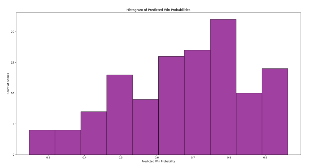
This histogram shows the frequency of our model’s predicted win probabilities. It best illustrates the model’s confidence throughout our dataset. We see this graph tends towards higher probabilities, the highest being 0.8 for over 20 games. If 0.5 was the most frequent, that means the model has virtually no confidence; it’s shrugging its shoulders and giving a random guess.
The histogram is best compared with the calibration curve. The former measures the distribution of predictions while the latter measures the quality of the predictions
Confusion Matrix
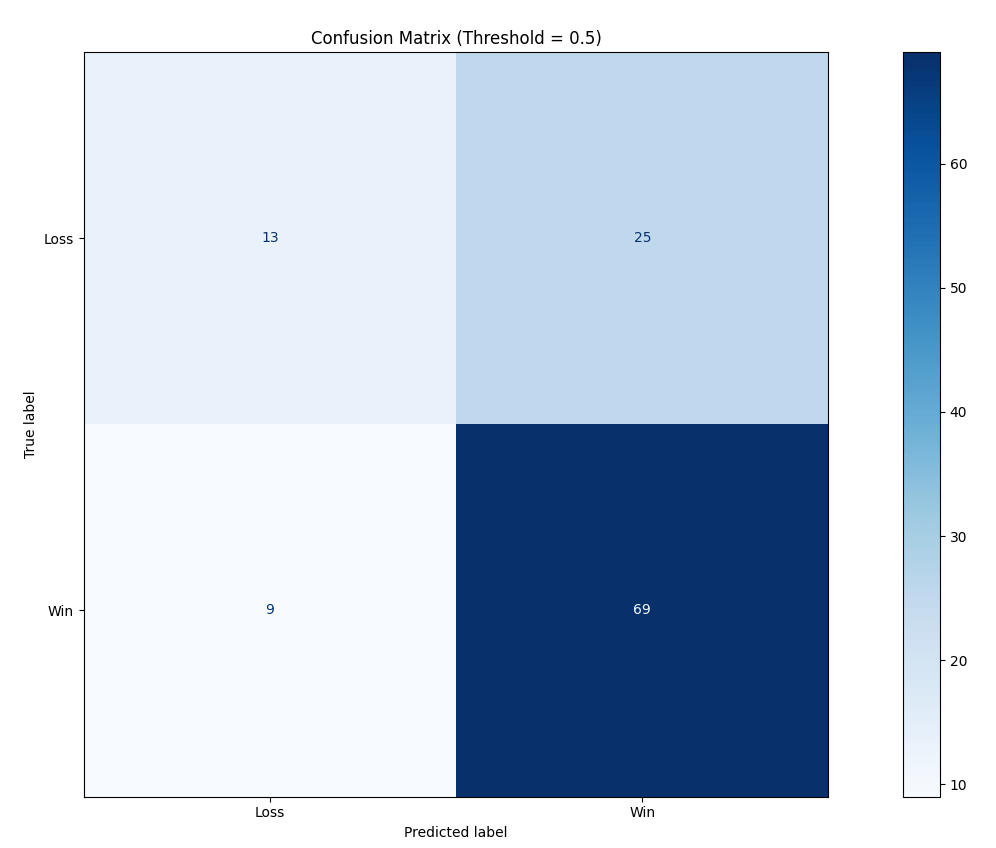
This confusion matrix is my personal favorite visualization out of the all the others. No percentages, no esoteric log-odds or advanced math needed to understand it. This is a simple 2×2 matrix that illustrates how many times the model was right and how often it was wrong.
The x-axis is the model’s win/loss predictions and the y-axis are the actual results. The bottom two squares are all the actual wins, and the top 2 are the losses.
The bottom-left-square means the model predicted a loss, but turned out to be a win, of which this happened 9 times. The bottom-right square shows that out of the 116 total games, the model correctly predicted a win 69 times, which is slightly above average accuracy.
So whether the model predicted a win or a loss, if the result matches the prediction, that’s a true prediction, meaning the model was correct. If it predicts win, and the result was a win, that’s a true positive. If it predicts a loss and the game was a loss, that’s a true negative, which healthily realistic. If it predicted a win but the result was a loss, that’s a false positive, which means the model was too optimistic. If it predicted a loss but turned out to be a win, that’s a false negative, meaning it was too doubtful.
This matrix is tuned for a 0.5 threshold, meaning any predicted probability at or above 0.5 is considered a win. We could of course tune this to be higher, say at 0.6 and any prediction lower is considered a loss.
Conclusion
Just using 3rd down conversion rates and total offensive yards, we were able to build a statistical model that predicts the probability of the Ravens winning a game. 3rd down conversion rate emerged as the stronger predictor. The model’s pseudo R2 of ≈0.12 shows the model is better than just guessing, but still far from perfect. Again, football games within seasons are relatively spaced out compared to baseball and basketball. So given the small sample size, the data can only be so precise, especially when only using two predictors. I just kept this simple for my first end-to-end statistical analysis project.
