Introduction
What determines how much we really need something? If we can’t get something we need, do we seek an alternative, or just do without?
At just about any grocery store you walk into, you’ll notice the bread, milk, and eggs aisles are usually towards the back. This is because they are the staples of our food consumption. You’ll seldom find anybody who does not consume at least one of these products. If the stores placed these at the front, people would walk in, instantly see and get what they need, and walk back out. They place these at the back to force you to walk through the store and see the other products before you reach the essentials. Given that these are essentials, that implies that people will buy them regardless of how much they cost right?
This is a question of price elasticity of demand. In this project, we will use real price data for each staple as well as income data in order to estimate how sensitive the demand for bread, milk, and eggs is to changes in price.
Data Collection
To start, we’ll be collecting two sets of data for each product: the average price, and pounds of consumption per capita.
We’ll also be downloading a dataset on household income so we can integrate it with our grocery features
For the average price, our primary source will be the Federal Reserve Bank St Louis (aka. FRED, economic data). The Bureau of Labor Statistics (BLS) has the same dataset, yet we’ll choose FRED’s since it only has two columns which are conveniently the most relevant, month/year, and average price per unit. BLS has a few extra columns that don’t add to the analysis.
The primary source for the consumption per capita data will be the USDA.
Let’s start with the price data. Go to the FRED website. On the right side of the homepage under ‘Browse Data By:’, click ‘Category’
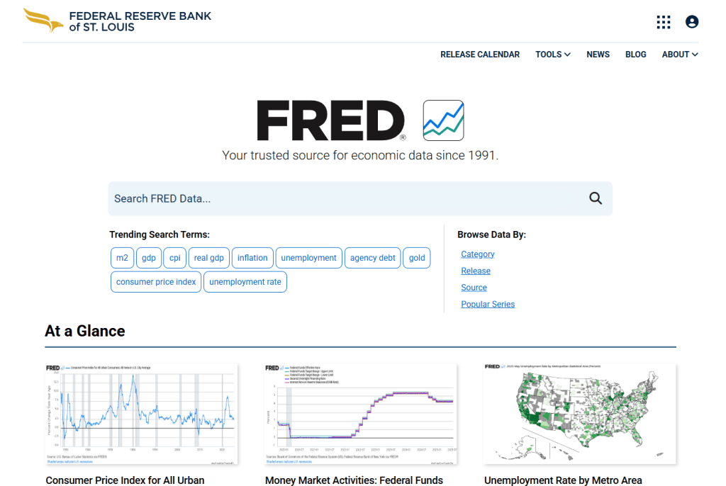
Scroll down (may have to first click ‘Category’) to the ‘Prices’ section and click ‘Commodities’

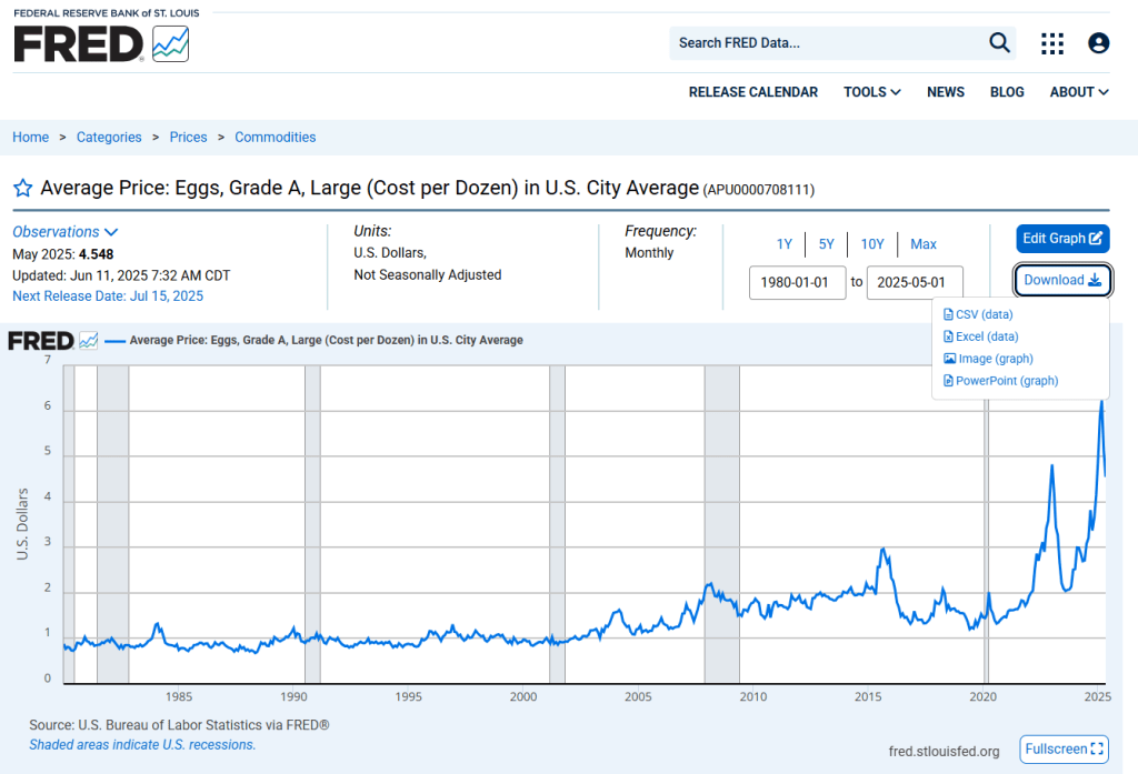
All 3 of our datasets should be on the first page. ‘Average Price’ for eggs, bread, and milk. Click and open all 3
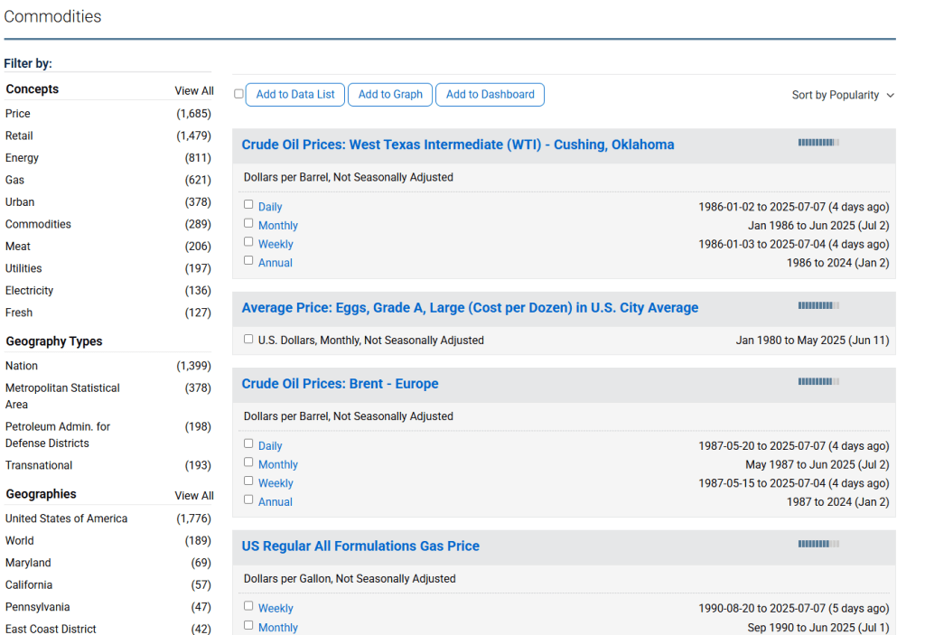
For each dataset, click on ‘Download’ and download it as a CSV file
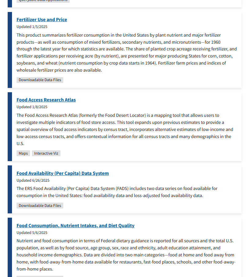
Next we’ll do our pounds per capita data. Go to the Economic Research Service branch of the USDA website. Scroll down a little to the box that says ‘Data’ and click ‘Explore All Data’

Scroll down to ‘Food Availability (Per Capita) Data System’ and click on that.
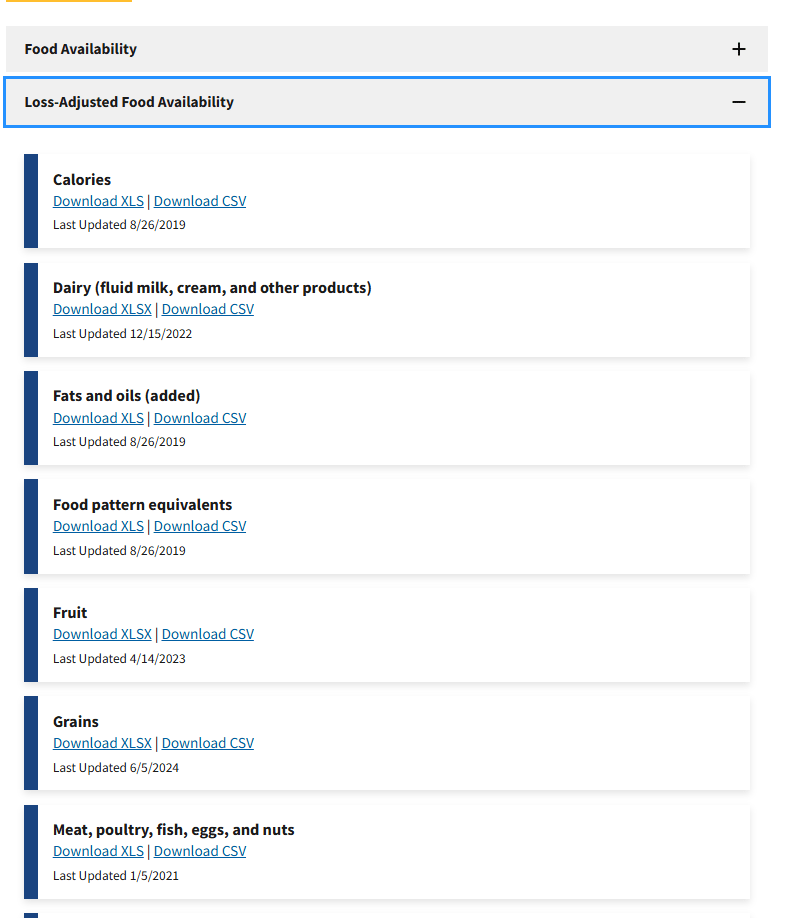
Now on this page, scroll all the way down to ‘Loss-Adjusted Food Availability’. Click the drop box, and now we see the main categories of foods. For this project, we’ll be downloading Dairy, Grains, and Meat; all as CSV files.
Household Income Data
Along with the average price and consumption data, we will also be including average household income. This takes our model from a simple price-quantity to a realistic demand system. Without this, we would only assume ‘price goes up, demand goes down’, which is a bit too black and white.
We’ll be taking our data from the US Census Bureau. This link should take you directly to the income. Download Table A-2.

HOW ALL DATA IS COLLECTED
It is important to remember that just about any dataset is a limited proxy/estimation for its subject(s). Even government agencies can only do so much in terms of collecting and organizing data. Not every single action that occurs in this world is recorded, nor should they be. There is not much more to say past this that will strengthen this analysis. If you are interested in the minute details of how any of the data used was collected and organized, the following are links to their sources’ documentations:
USDA Food Availability (Per Capita) Data System: https://www.ers.usda.gov/data-products/food-availability-per-capita-data-system/food-availability-documentation
Census 2025 Annual Social and Economic (ASEC) Supplement: https://www2.census.gov/programs-surveys/cps/techdocs/cpsmar25.pdf
Bureau of Labor Statistics (BLS): https://www.bls.gov/opub/hom/cpi/home.htm
Preprocessing
Now that we have our data downloaded, we have to prepare them for analysis.
The big issue we have is that the price data is monthly, yet the consumption data is yearly. This means we have to stick with our lowest common denominator, which is yearly.
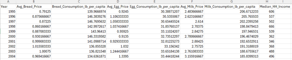
import osimport pandas as pd# ============= Paths =============MAIN_FOLDER = r"C:\Users\username\data\Economics"income_file = os.path.join(MAIN_FOLDER, "Median_HH_Income_1995_2019.xlsx")# ============= Load raw price data =============bread_price = pd.read_csv(os.path.join(MAIN_FOLDER, "Average Price of Bread.csv"))eggs_price = pd.read_csv(os.path.join(MAIN_FOLDER, "Average Price of Eggs.csv"))milk_price = pd.read_csv(os.path.join(MAIN_FOLDER, "Average Price of Milk.csv"))# ============= Load consumption data =============loss_meat = pd.read_csv(os.path.join(MAIN_FOLDER, "LossAdj - meat.csv"))loss_dairy = pd.read_csv(os.path.join(MAIN_FOLDER, "LossAdj - Dairy.csv"))loss_grain = pd.read_csv(os.path.join(MAIN_FOLDER, "LossAdj - grain.csv"))# ============= Normalize price dates -> Year =============for df in (bread_price, eggs_price, milk_price): df['observation_date'] = pd.to_datetime(df['observation_date'], errors='coerce') df['Year'] = df['observation_date'].dt.year# Yearly averagesbread_price_clean = ( bread_price.groupby('Year', as_index=False)['Cost Per Pound'] .mean().rename(columns={'Cost Per Pound': 'Avg_Bread_Price'}))eggs_price_clean = ( eggs_price.groupby('Year', as_index=False)['Cost per dozen'] .mean().rename(columns={'Cost per dozen': 'Avg_Egg_Price'}))milk_price_clean = ( milk_price.groupby('Year', as_index=False)['Cost per gallon'] .mean().rename(columns={'Cost per gallon': 'Avg_Milk_Price'}))# ============= Filter consumption series =============eggs_cons = ( loss_meat[ (loss_meat['Commodity'].str.startswith('Eggs: Per capita availability adjusted for loss')) & (loss_meat['Attribute'] == 'Primary weight-Lbs/year') ][['Year', 'Value']] .rename(columns={'Value': 'Egg_Consumption_lb_per_capita'}))milk_cons = ( loss_dairy[ (loss_dairy['Commodity'] == 'All beverage milks: Per capita availability adjusted for loss') & (loss_dairy['Attribute'] == 'Primary weight-Lbs/year') ][['Year', 'Value']] .rename(columns={'Value': 'Milk_Consumption_lb_per_capita'}))bread_cons = ( loss_grain[ (loss_grain['Commodity'].str.startswith('Wheat flour: Per capita availability adjusted for loss')) & (loss_grain['Attribute'] == 'Primary weight-Lbs/year') ][['Year', 'Value']] .rename(columns={'Value': 'Bread_Consumption_lb_per_capita'}))# ============= Merge staples panels =============merged = ( bread_price_clean.merge(bread_cons, on='Year', how='inner') .merge(eggs_price_clean, on='Year', how='inner') .merge(eggs_cons, on='Year', how='inner') .merge(milk_price_clean, on='Year', how='inner') .merge(milk_cons, on='Year', how='inner'))# ============= Load & clean Household Income (Census) =============income_raw = pd.read_excel(income_file, header=None) # no headers; treat all rows as dataincome_raw = income_raw.iloc[6:, :].copy() # skip top header rows (first valid years start at row 7)# Extract 4-digit year from column 0; drop rows without a yearincome_raw['Year'] = income_raw.iloc[:, 0].astype(str).str.extract(r'(\d{4})', expand=False)income_raw = income_raw.dropna(subset=['Year'])income_raw['Year'] = income_raw['Year'].astype(int)# Try to locate Median income (estimate) column robustly.# Typical positions: total ~15 columns; Median(Estimate) is often col index 11 (0-based) or -4.median_col = Nonecandidate_idxs = [-4, 11, 12] # try common positions firstfor idx in candidate_idxs: if -income_raw.shape[1] <= idx < income_raw.shape[1]: s = pd.to_numeric(income_raw.iloc[:, idx], errors='coerce') if s.notna().sum() >= 30: median_col = idx break# Fallback: pick the numeric column with most values in a sensible income rangeif median_col is None: num = income_raw.apply(pd.to_numeric, errors='coerce') # Count entries that look like incomes (10k–200k) scores = num.apply(lambda s: s.between(10_000, 200_000).sum()) median_col = scores.idxmax()income_raw['Median_HH_Income'] = pd.to_numeric(income_raw.iloc[:, median_col], errors='coerce')# Keep the FIRST occurrence of each year in sheet order -> corresponds to ALL RACES blockincome_raw['year_first'] = income_raw.groupby('Year').cumcount()income_df = income_raw.loc[income_raw['year_first'] == 0, ['Year', 'Median_HH_Income']].copy()# Drop rows with no income value (rare but safe)income_df = income_df.dropna(subset=['Median_HH_Income'])# ============= Merge income into staples panel =============merged = merged.merge(income_df, on='Year', how='inner')# ============= Finalize & export =============merged = merged.sort_values('Year').drop_duplicates(subset='Year')output_path = os.path.join(MAIN_FOLDER, "Staples_Merged_With_Income.csv")merged.to_csv(output_path, index=False)print("Final merged file with household income saved to:")print(output_path)Analysis Code
Full Script
import os
import numpy as np
import pandas as pd
import statsmodels.api as sm
import matplotlib.pyplot as plt

# ===== Paths =====
MAIN_FOLDER = r"C:\Users\username\GroceryStaples"
MERGED_FILE = os.path.join(MAIN_FOLDER, "Staples_Merged_With_Income.csv")

# ===== Load merged wide dataset (Year-level, prices, quantities, income) =====
df_wide = pd.read_csv(MERGED_FILE)


# ===== Show income trend =====
plt.figure(figsize=(9, 4.5))
plt.plot(df_wide["Year"], df_wide["Median_HH_Income"], marker="o")
plt.title("Median Household Income (CPI-Adjusted) – All Races")
plt.xlabel("Year")
plt.ylabel("Dollars")
plt.grid(True)
plt.tight_layout()
plt.show()

# ===== Reshape to long form: (Year, Food, Price, Quantity, Income) =====
spec = [
    ("Bread", "Avg_Bread_Price", "Bread_Consumption_lb_per_capita"),
    ("Eggs",  "Avg_Egg_Price",   "Egg_Consumption_lb_per_capita"),
    ("Milk",  "Avg_Milk_Price",  "Milk_Consumption_lb_per_capita"),
]

parts = []
for food, pcol, qcol in spec:
    sub = df_wide[["Year", pcol, qcol, "Median_HH_Income"]].copy()
    sub.columns = ["Year", "Price", "Quantity", "Median_HH_Income"]
    sub["Food"] = food
    parts.append(sub)

df = pd.concat(parts, ignore_index=True)
df.to_csv("Staples_Long_Format.csv", index=False)


#Sort rows by Food and Year
df = df.sort_values(["Food", "Year"])

# ===== Run elasticity regressions and plot =====
foods = ["Bread", "Eggs", "Milk"]
fig, axes = plt.subplots(3, 4, figsize=(24, 12))  # 4th col = income panel
fig.suptitle("Elasticity Analysis with Household Income: Bread, Eggs, Milk", fontsize=18)

results = []

for i, food in enumerate(foods):
    sub = df[df["Food"] == food].copy()

    # Derived fields
    sub["Revenue"] = sub["Price"] * sub["Quantity"]
    sub["log_Q"] = np.log(sub["Quantity"])
    sub["log_P"] = np.log(sub["Price"])
    sub["log_Y"] = np.log(sub["Median_HH_Income"])

    X = sm.add_constant(sub[["log_P", "log_Y"]])
    y = sub["log_Q"]
    model = sm.OLS(y, X, missing="drop").fit()

    # Collect key metrics
    bP = model.params.get("log_P", np.nan)
    bY = model.params.get("log_Y", np.nan)
    ci = model.conf_int()
    ciP = ci.loc["log_P"].tolist() if "log_P" in ci.index else [np.nan, np.nan]
    ciY = ci.loc["log_Y"].tolist() if "log_Y" in ci.index else [np.nan, np.nan]
    results.append({
        "Food": food,
        "Obs": int(model.nobs),
        "R2": model.rsquared,
        "PriceElasticity": bP, "PE_CI_low": ciP[0], "PE_CI_high": ciP[1], "PE_p": model.pvalues.get("log_P", np.nan),
        "IncomeElasticity": bY, "IE_CI_low": ciY[0], "IE_CI_high": ciY[1], "IE_p": model.pvalues.get("log_Y", np.nan)
    })

    # Console summary
    print(f"\n\n========= {food} Elasticity Model =========")
    print(model.summary())

#VISUALIZATIONS

    # ---- Col 1: Actual vs Predicted log(Q) ----
    sub["Pred_log_Q"] = model.predict(X)
    ax1 = axes[i, 0]
    ax1.plot(sub["Year"], sub["log_Q"], marker="o", label="Actual")
    ax1.plot(sub["Year"], sub["Pred_log_Q"], marker="x", label="Predicted")
    ax1.set_title(f"{food} - Actual vs Predicted log(Q)")
    ax1.set_xlabel("Year")
    ax1.set_ylabel("log(Q)")
    ax1.grid(True)
    ax1.legend()

       # ---- Col 2: Per-capita annual spending trend ($/person/year) ----
    ax2 = axes[i, 1]
    ax2.plot(sub["Year"], sub["PerCapitaSpending"], marker="o")
    ax2.set_title(f"{food} - Per-Capita Spending Trend")
    ax2.set_xlabel("Year")
    ax2.set_ylabel("$/person/year")
    ax2.yaxis.set_major_formatter(FuncFormatter(lambda v, _: f"${v:,.0f}"))
    ax2.grid(True)

    # ---- Col 3: Demand curve (log Q vs log P) at mean income ----
    mean_income = sub["log_Y"].mean()
    price_range = np.linspace(sub["log_P"].min(), sub["log_P"].max(), 50)
    demand_curve = (
        model.params.get("const", 0.0)
        + model.params.get("log_Y", 0.0) * mean_income
        + model.params.get("log_P", 0.0) * price_range
    )
    ax3 = axes[i, 2]
    ax3.scatter(sub["log_P"], sub["log_Q"], alpha=0.6, label="Observed")
    ax3.plot(price_range, demand_curve, label="Fitted")
    ax3.set_title(f"{food} - Demand vs Price (log-log)")
    ax3.set_xlabel("log(Price)")
    ax3.set_ylabel("log(Quantity)")
    ax3.grid(True)
    ax3.legend()

    # ---- Col 4: Income response (log Q vs log Y) at mean price ----
    mean_price = sub["log_P"].mean()
    inc_grid = np.linspace(sub["log_Y"].min(), sub["log_Y"].max(), 50)
    inc_curve = (
        model.params.get("const", 0.0)
        + model.params.get("log_P", 0.0) * mean_price
        + model.params.get("log_Y", 0.0) * inc_grid
    )
    ax4 = axes[i, 3]
    ax4.scatter(sub["log_Y"], sub["log_Q"], alpha=0.6, label="Observed")
    ax4.plot(inc_grid, inc_curve, label="Fitted")
    ax4.set_title(f"{food} - Demand vs Income (log-log)")
    ax4.set_xlabel("log(Income)")
    ax4.set_ylabel("log(Quantity)")
    ax4.grid(True)
    ax4.legend()

plt.tight_layout(rect=[0, 0, 1, 0.95])
plt.show()

# ===== Elasticity summary table =====
df_results = pd.DataFrame(results)
print("\n\n=== Elasticity Summary (price & income) ===")
print(df_results)

out_res = os.path.join(MAIN_FOLDER, "Staples_Elasticity_Summary.csv")
df_results.to_csv(out_res, index=False)
print("Saved:", out_res)
Line-by-Line Analysis
import osimport numpy as npimport pandas as pdimport statsmodels.api as smimport matplotlib.pyplot as plt# ===== Paths =====MAIN_FOLDER = r"C:\Users\username\Grocery Staples"MERGED_FILE = os.path.join(MAIN_FOLDER, "Staples_Merged_With_Income.csv")We start with importing a handful of libraries.
- os is for navigating file paths
- numpy is for advanced math functions
- pandas is for handling spreadsheets
- statsmodels.api is for our OLS regression model
- matplotlib.pyplot is for plotting
- The MAIN_FOLDER and MERGED_FILE variables point to our preprocessed file
df_wide = pd.read_csv(MERGED_FILE)df_wide loads in the dataset.
plt.figure(figsize=(9, 4.5))plt.plot(df_wide["Year"], df_wide["Median_HH_Income"], marker="o")plt.title("Median Household Income (CPI-Adjusted) – All Races")plt.xlabel("Year")plt.ylabel("Dollars")plt.grid(True)plt.tight_layout()plt.show()Before we move on to the grocery staples, we’re first going to create our visualization for national income trend. This is where we use the median household income data. We first plot CPI-adjusted median household income over time to show the macro context for the income variable used in the regressions.
# ===== Reshape to long form: (Year, Food, Price, Quantity, Income) =====spec = [ ("Bread", "Avg_Bread_Price", "Bread_Consumption_lb_per_capita"), ("Eggs", "Avg_Egg_Price", "Egg_Consumption_lb_per_capita"), ("Milk", "Avg_Milk_Price", "Milk_Consumption_lb_per_capita"),]parts = []for food, pcol, qcol in spec: sub = df_wide[["Year", pcol, qcol, "Median_HH_Income"]].copy() sub.columns = ["Year", "Price", "Quantity", "Median_HH_Income"] sub["Food"] = food parts.append(sub)df = pd.concat(parts, ignore_index=True)df.to_csv("Staples_Long_Format.csv", index=False)The dataset is currently in wide form. Meaning each year get its own row and within that row we have each staple’s average price and consumption per capita, along with the median household income at the end.
Though this doesn’t seem like much to us visually, this means when the statistical model runs, it will be doing an analysis for each of the staples which is redundant, a waste of code space, and a waste of computing power. By converting this to long form, we’ll be able to loop all of the staples into one block of code; we get the same result with less code, and it’ll execute faster.
spec = [ ("Bread", "Avg_Bread_Price", "Bread_Consumption_lb_per_capita"), ("Eggs", "Avg_Egg_Price", "Egg_Consumption_lb_per_capita"), ("Milk", "Avg_Milk_Price", "Milk_Consumption_lb_per_capita"),]spec is a list of 3 tuples. This helps us contain each staple’s two columns into a single variable. Now we only have to call 3 variables instead of 6.
parts = []parts is an empty list where the 3 staples will stack
for food, pcol, qcol in spec: sub = df_wide[["Year", pcol, qcol, "Median_HH_Income"]].copy() sub.columns = ["Year", "Price", "Quantity", "Median_HH_Income"] sub["Food"] = food parts.append(sub)The dataset is originally in wide format, with separate price and quantity columns for each staple. We reshape it into long format so that all staples share common fields (Price, Quantity, Income) and are distinguished by a Food identifier. This allows a single modeling loop to estimate elasticity consistently across goods.
df = pd.concat(parts, ignore_index=True)This is the final connector that makes our dataset from wide to long form.
df.to_csv("Staples_Long_Format.csv", index=False)I added this line to create a file where we can see the change in the dataset. This is NOT an analysis and this line is NOT mandatory. We are simply rearranging the data so the model can iterate through it smoother. If you leave this line out, the rearrangement will still happen. It’ll just be behind the scenes.
#Sort rows by Food and Yeardf = df.sort_values(["Food", "Year"])This sort_values method sorts our rows in order from earliest to latest year. We want this in chronological order to the stat model and execute properly with no hiccups. Getting our ducks in a row
# ===== Run elasticity regressions and plot =====foods = ["Bread", "Eggs", "Milk"]fig, axes = plt.subplots(3, 4, figsize=(24, 12)) # 4th col = income panelfig.suptitle("Elasticity Analysis with Household Income: Bread, Eggs, Milk", fontsize=18)- We start with a list of our staples Bread Milk and Eggs that we’ll set to a variable foods. This will drive the loop of the analysis.
- This block initializes the graphs we’ll be looking at. The subplots method starts us off by creating 3 rows and 4 columns, which is 12 subplots. We’ll set their sizes as 24×12 which will make them big enough to read but not so big they overlap. After that is just a comment so that we keep in mind the 4th column is meant for the income panels.
- suptitle is the super title, the main title of the graph along with its font size.
results = []for i, food in enumerate(foods): sub = df[df["Food"] == food].copy()- This results variable create an empty container that we’ll store our summary info from each regression.
- Next we initialize the loop with i which indexes each staple (Bread is 0, Eggs is 1, and Milk is 2) so that it selects all of its information for its analysis, which is what the == does as well.
# Derived fields sub["Revenue"] = sub["Price"] * sub["Quantity"] sub["log_Q"] = np.log(sub["Quantity"]) sub["log_P"] = np.log(sub["Price"]) sub["log_Y"] = np.log(sub["Median_HH_Income"]) X = sm.add_constant(sub[["log_P", "log_Y"]]) y = sub["log_Q"] model = sm.OLS(y, X, missing="drop").fit()This section creates new columns that we’ll be using. Some for analysis, and some will be plotted.
- The first ‘Revenue’ column is created by multiplying Price and Quantity. This will be used to plot spending trends.
- log_Q = dependent variable
- log_P = price elasticity
- log_Y = income elasticity
- The regression includes an intercept term to allow for a baseline level of demand independent of price and income.
Mathematically, this block is setting up the regression: logQ = β0 + βPlogP + βYlogY + ε
# Collect key metrics bP = model.params.get("log_P", np.nan) bY = model.params.get("log_Y", np.nan) ci = model.conf_int() ciP = ci.loc["log_P"].tolist() if "log_P" in ci.index else [np.nan, np.nan] ciY = ci.loc["log_Y"].tolist() if "log_Y" in ci.index else [np.nan, np.nan] results.append({ "Food": food, "Obs": int(model.nobs), "R2": model.rsquared, "PriceElasticity": bP, "PE_CI_low": ciP[0], "PE_CI_high": ciP[1], "PE_p": model.pvalues.get("log_P", np.nan), "IncomeElasticity": bY, "IE_CI_low": ciY[0], "IE_CI_high": ciY[1], "IE_p": model.pvalues.get("log_Y", np.nan) })After estimating the model, we extract key metrics for reporting:
– Price elasticity and income elasticity
– Their confidence intervals
– p-values for hypothesis testing
– R² (model fit)
– Number of observations
These are compiled into a summary table for comparison across staples.
print(f"\n\n========= {food} Elasticity Model =========")print(model.summary())Then lastly we print the summary of the model along with its title above it.
And that is all the code for the model itself. Everything after pertains to the visualizations
Key Results
Of all of these resulting terms, there are only five that tell the full story.
Because the model is log–log, both coefficients represent the % change in quantity, just in response to a different feature. is the change in response to price, and is the change in response to income:
- represents the % change in quantity for a 1% change in price
- represents the % change in quantity for a 1% change in income
Again,
- Elastic (> 1): consumers respond strongly
- Inelastic (< 1): consumers respond weakly
- Negative: price and quantity move in opposite directions
Bread
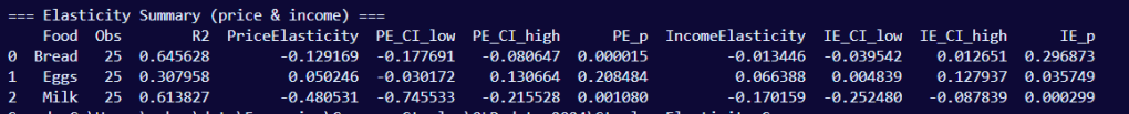
Price elasticity’s (log_P) coefficient is -0.1292 (p < 0.001) indicating that bread demand is price inelastic. A 1% price increase is associated with an almost 0.13% decrease in quantity demanded, meaning consumers are relatively unresponsive to price changes in bread. Income elasticity (log_Y) is -0.013 (p = 0.297) which is statistically undistinguishable from zero, indicating that changes in household income has no significant affect on bread consumption. Given that both of these variables resulted in minimal change in consumption, this concludes that bread is a staple good; people will always buy bread regardless of the economy.
Together, price and income explain 64.6% (R2 = 0.646) of the variation in bread. This means the model captures a substantial portion of observed behavior. An F-test rejects the null hypothesis that price and income jointly have no explanatory power (F = 20.04, p < 0.001), confirming that the model as a whole provides meaningful information beyond a baseline model with no predictors. All estimates are based on 25 annual observations.
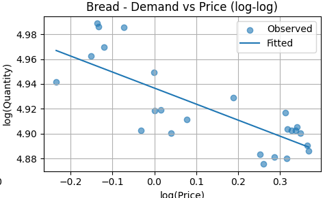
The fitted line slopes downward, consistent with the estimated negative price elasticity. The slope is shallow, indicating that quantity responds only modestly to price changes across the observed range. The scatter around the fitted line suggests a stable but weak inverse relationship, reinforcing bread’s inelastic demand.
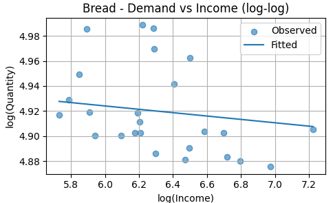
The fitted line is nearly flat, indicating little to no systematic relationship between income and bread consumption within the observed variation. This visual pattern supports the regression result that bread’s income elasticity is close to zero and not statistically distinguishable from zero. In practical terms, changes in household income do not meaningfully shift bread demand in this sample.
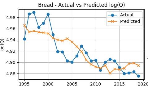
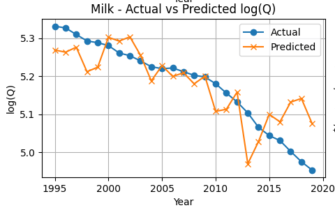
The predicted series tracks the observed log(quantity) closely over time, capturing the broad consumption pattern with relatively small deviations. This alignment visually supports the model’s reported explanatory power and suggests that the estimated price and income effects jointly produce plausible demand predictions year by year.
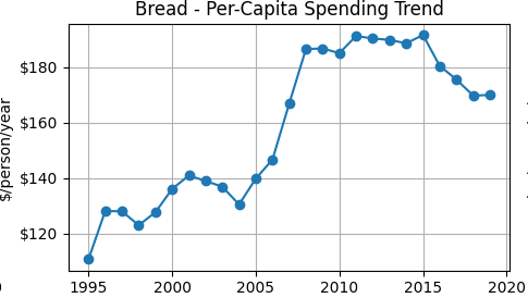
Per-capita spending on bread rises through the mid-2000s, remains elevated into the early 2010s, and then moderates slightly in later years. For inelastic goods, spending can rise even if quantity declines because price increases dominate the relatively small quantity response. This trend is consistent with the estimated inelastic price elasticity and provides an intuitive complement to the regression results.
Eggs
Price elasticity for eggs (log_P) is 0.0502 (p = 0.208), which is statistically indistinguishable from zero, indicating that egg consumption does not respond meaningfully to price changes over the sample period. Income elasticity (log_Y) is 0.0664 (p = 0.036), which is positive and statistically significant, indicating that a 1% increase in income is associated with roughly a 0.07% increase in egg consumption. This suggests that eggs behave as a weak normal good, with consumption rising modestly as income increases.
Together, price and income explain 30.8% (R² = 0.308) of the variation in egg consumption, indicating moderate explanatory power. An F-test rejects the null hypothesis that price and income jointly have no explanatory power (F = 4.90, p = 0.017), confirming that the model provides meaningful information beyond a baseline model with no predictors. All estimates are based on 25 annual observations.
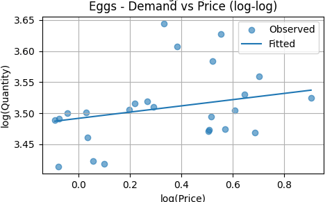
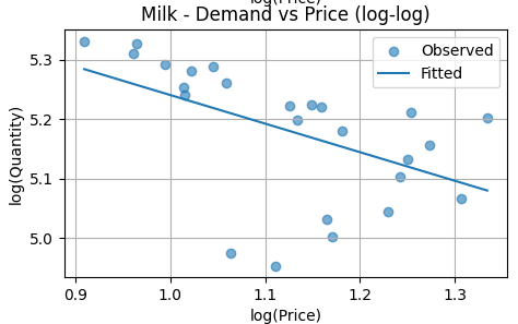
The fitted line slopes slightly upward, indicating a small positive price coefficient. However, the relationship is weak and statistically insignificant. The scattered points show no clear downward pattern, meaning egg demand does not respond strongly to price changes in this sample. This aligns with the regression result that price elasticity for eggs is not statistically different from zero.
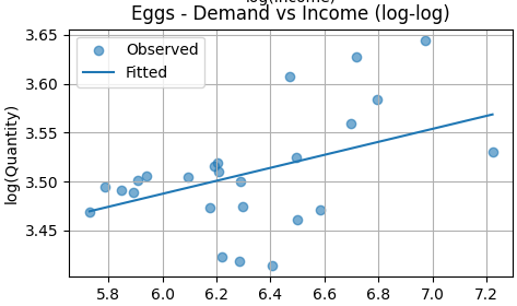
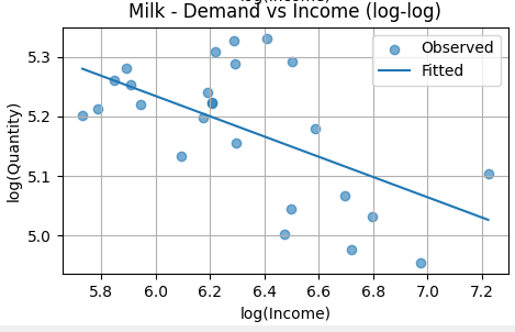
The fitted line slopes upward and is statistically significant. This indicates that higher income is associated with higher egg consumption. Eggs behave as a normal good in this dataset, with a modest but meaningful income elasticity.
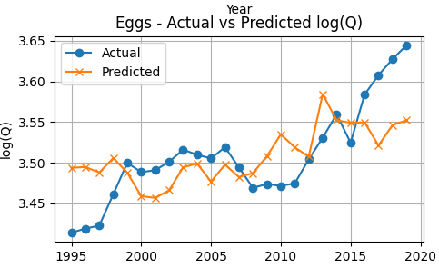
Egg consumption shows a gradual upward trend over time. The model tracks the general direction of this increase, though deviations are visible in several years. The widening gap in later years suggests that factors beyond price and income may be influencing egg demand. Overall, the model captures the trend but explains a modest portion of the variation (consistent with the lower R²).
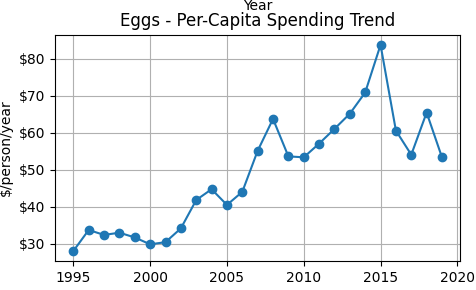
Per-capita egg spending rises steadily from the late 1990s through the mid-2010s, peaking around 2015 before declining. The upward trend reflects either higher prices, greater consumption, or both. This visual supports the positive income elasticity found in the regression results, as spending growth coincides with broader economic expansion.
Milk
Price elasticity for milk (log_P) is -0.4805 (p = 0.001), indicating that milk demand is price inelastic but substantially more responsive than bread. A 1% increase in price is associated with an approximately 0.48% decrease in quantity demanded. Income elasticity (log_Y) is −0.1702 (p < 0.001), indicating that higher income is associated with lower milk consumption, consistent with milk behaving as an inferior or substitutable staple as consumers shift toward alternatives.
Together, price and income explain 57.9% (R² = 0.579) of the variation in milk consumption, showing strong explanatory power. An F-test rejects the null hypothesis that price and income jointly have no explanatory power (F = 17.48, p < 0.001), confirming that the model provides meaningful information beyond a baseline model with no predictors. All estimates are based on 25 annual observations.
The fitted line slopes downward and is statistically significant. This confirms that milk demand is price elastic relative to bread and eggs. As price increases, quantity demanded decreases in a clear and economically meaningful way.
The fitted line slopes downward and is statistically significant. This indicates negative income elasticity. Milk behaves as an inferior good in this sample: as income rises, milk consumption declines.
Milk consumption trends downward over time. The model tracks this decline closely, particularly in the early and middle years, though deviations appear during periods of volatility. The fit is stronger than for eggs, consistent with the higher explanatory power in the regression.
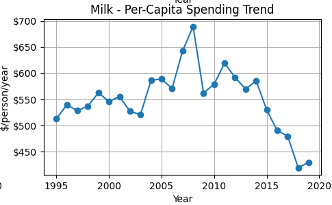
Milk spending peaks in the late 2000s and then declines sharply after 2014. This suggests falling consumption, falling prices, or both. The decline in spending mirrors the downward trend in quantity demanded shown in the log(Q) graph.
Comparative Synthesis
The three staples behave very differently from each other. Bread is almost completely unresponsive to both price and income changes – people buy it regardless of what’s happening in the economy. It’s a true necessity with a price elasticity of just -0.12 and essentially zero income effect.
Eggs fall somewhere in the middle. Price changes don’t move the needle much, but there’s a small positive income elasticity. As people earn more, they buy slightly more eggs – making eggs a normal good, just not a strong one.
Milk is the outlier. It’s still technically inelastic, but at -0.48, it’s about four times more price-responsive than bread. Even more interesting: milk has a negative income elasticity of -0.17. As people get richer, they actually buy less milk, probably switching to alternatives like plant-based beverages or other drinks.
The models tell different stories too. Price and income explain about 65% of bread consumption and 58% of milk consumption – pretty solid. But for eggs? Only 31%. Something else is driving egg purchases beyond just price and household income.
The takeaway: you can’t lump all staples together. Even among basic grocery items everyone buys, the way people respond to price and income changes varies a lot depending on the product.
Methodology
Data and Variables
We analyze annual data on grocery staples. For each year , quantity demanded () is measured as per-capita consumption, price () as the average market price, and income () as median household income. The sample consists of 25 annual observations drawn from publicly available aggregate data sources. Using per-capita quantities allows demand to be examined independently of population growth.
Elasticity Framework
The objective is to estimate how responsive quantity demanded is to changes in price and income. Responsiveness is naturally defined in percentage terms, making elasticity the appropriate measure. For example, a price elasticity of −0.5 would indicate that a 10% increase in price leads to a 5% decrease in quantity demanded. This framework is particularly suitable for staple goods, where proportional responses are more informative than absolute changes.
Log–Log Specification
To estimate elasticities directly, all variables are transformed using natural logarithms. Taking logarithms of both sides converts percentage changes into a linear relationship that can be estimated using standard regression methods. In this log–log specification, coefficients can be interpreted directly as elasticities.
Model Specification
Demand is estimated using the following regression model:
Here, represents the price elasticity of demand and represents the income elasticity of demand. The error term captures unobserved factors affecting demand, including random variation and measurement error.
Estimation Method and Identification
Model parameters are estimated using Ordinary Least Squares (OLS). Identification relies on the assumption that year-to-year variation in prices is driven primarily by supply-side factors such as input costs, production conditions, and broader market forces; rather than contemporaneous demand shocks. Under this assumption, OLS provides consistent estimates of demand elasticities. While price and quantity are jointly determined in theory, this approach is standard in aggregate demand estimation when richer instruments are unavailable and results are interpreted as conditional associations rather than structural causal effects.
Demand Curve Construction
To visualize the implied demand relationship, income is held constant at its sample median while price is varied over its observed range. Predicted quantities are then computed using the estimated coefficients, yielding a demand curve that reflects the model’s estimated price responsiveness for each good separately.
Limitations
This analysis uses aggregate annual data and a reduced-form demand specification, which limits causal interpretation. Prices and quantities are jointly determined in theory, and while identification relies on the assumption that year-to-year price variation is driven primarily by supply-side factors, unobserved demand shocks may still bias estimates. Additionally, demand for eggs and milk appears influenced by factors beyond price and income, such as dietary preferences and substitution toward alternatives, which are not captured in the model. These results should therefore be interpreted as descriptive demand relationships rather than structural causal estimates.
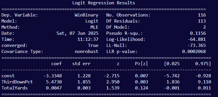
Interpretation of Results
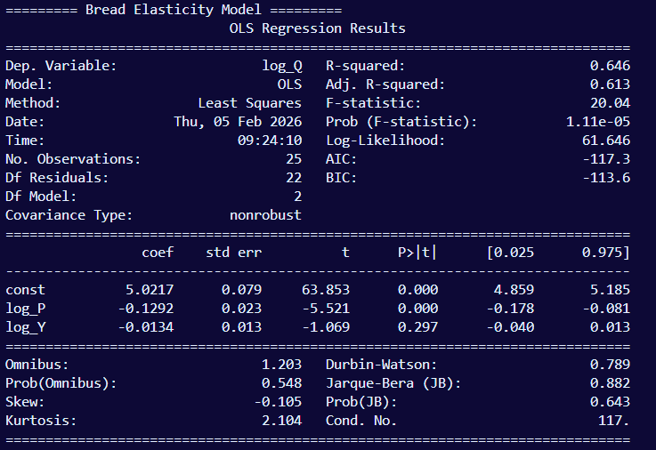
These are only the results of bread’s elasticity. The format is the same for eggs and milk.
- Dep. Variable: the dependent variable is log_Q (Quantity). This is the variable whose results we are observing while price and income do their natural fluctuations.
- Model: OLS (Ordinary Least Squares), the statistical model being estimated
- Method: Least Squares.
- This may seem redundant to #2 since OLS literally means Least Squares. The only distinction is that the Method is the estimation method that is applied to the model. In this case, the OLS model has a specific estimation method to go with it, so they do overlap. But other models have various estimation methods they can be paired with.
- This may seem redundant to #2 since OLS literally means Least Squares. The only distinction is that the Method is the estimation method that is applied to the model. In this case, the OLS model has a specific estimation method to go with it, so they do overlap. But other models have various estimation methods they can be paired with.
- Date & Time: Self-explanatory. This is when I ran the model that shown in the image
- No. Observations: The number of observations; in this case the number of snapshots of bread’s price and quantity, which is 25 years. This is the same for milk and eggs as well as household income.
- Degrees of freedom (Df) Residuals: This is the number of observation (25 years) minus our 2 predictors (2, as shown in Df Model below) minus an extra 1 to account for the intercept. This is a relatively small residual
- Df Model: the number of predictors used in the model. Price and household income, which is 2.
- Covariance type: this measures how well the standard errors were calculated. ‘nonrobust’ is the default value, meaning the model is correctly specified and errors meet all assumptions.
- R-squared: The value 0.646 means that using price and income reduces overall prediction error by about 64.6% compared to making a dumb prediction that always guesses the average.
- Adj. R-squared: Prevents R² from artificially increasing when you add variables.
- F-statistic: Tests whether the model as a whole is better than no model at all. It compares the implemented model with a baseline model with no predictors (intercept only)
- Prob (F-statistic): Quantify how surprising the F-statistic would be if the predictors were useless. The value -0.00001 means it is extremely unlikely that price and income jointly explain nothing.
- Log-Likelihood: Measure how plausible the observed data is under the model.
- Akaike Information Criterion (AIC): Balance fit vs complexity.
- Bayesian Information Criterion (BIC): Same as AIC, but harsher penalty for complexity.
Bottom Half
- Omnibus: Checks if the residuals roughly follow a normal distribution; a joint test of skewness and kurtosis. Since there are only 25 observations, this makes the omnibus test of lower power
- Prob(Omnibus): Assuming errors are normal, how significatn would observed skewness and kurtosis be? A high value would mean there is no strong evidence against normality, and a low value would indicate the errors are non-normal
- Skew: Measures if errors are symmetric around 0. A positive skew means it tends towards a long right tail, and a negative (which it is in this case) means it tends towards a long left tail
- Kurtosis: Measures how heavy are the tails of the error distribution? A value of 3 is normal-like, above 3 are heavy tails, and below 3 (which it is in this case) are light tails.
- Durbin-Watson: Checks if the errors are correlated over time. Do the positive errors tend to follow positive errors? Do the negative errors cluster?
- Jarque-Bera (JB): Checks if the residuals look approximately normal. Bigger is less normal; deviating from the normal shape. Smaller is more normal
- Prob(JB): Quantifies how the observed JB value would be if the residuals were truly normal; the p-value for the JB test to put it simply. Low (below 0.05) indicates non-normal residuals, and high means there is no strong evidence against normality
- Condition Number: Checks if the predictors are numerically well-behaved or nearly redundant. Below 30 is considered very safe. There is no concern for instability until it gets close to 1000. So our model’s result of 117 is acceptable.